how do keyword spotting models work?
a guide to keyword spotting, audio features, neural networks, training, and continuous detection
You have always used "Hey Siri," "Alexa," or "OK Google," but have you ever thought: how do they actually work? How does the phone know that they're being called right now?
This is done with the help of special models called keyword spotting models. Its task is not to transcribe everything the user says, but to detect a predefined word or a short phrase inside any audio stream. Since it does not even transcribe anything, it's significantly smaller, significantly faster, and runs continuously on our phones and every kind of on edge device.
The basic pipeline
Here is a rough diagram about how the pipeline works. We will go into detail about how each part works soon.
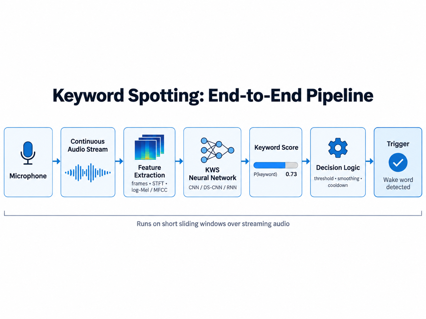
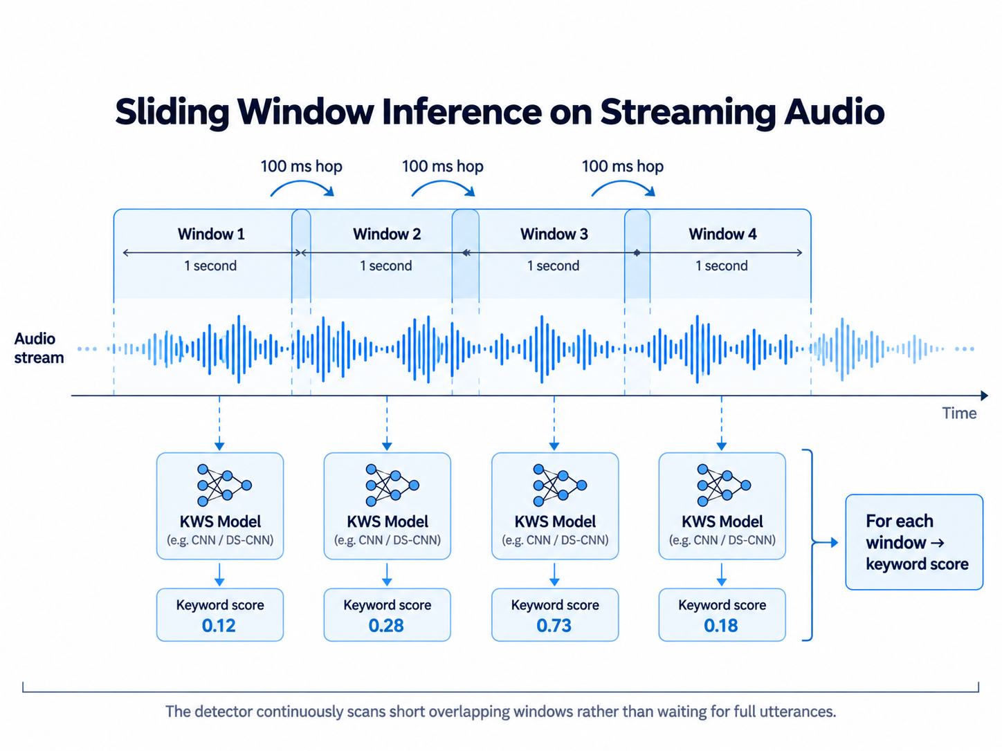
Suppose the wake word is "hey device." The microphone continuously records the audio, and usually it is recorded at 16 kHz. Instead of feeding a very long raw waveform directly to the model, the system will usually analyze a short sliding window, such as 1 second.
The model gets these small sliding window audios and asks, "Does this 1-second window contain my keyword?" This is very important because this kind of a detector cannot wait for the person to finish his or her complete sentence. It continuously needs to inspect what stream of audio is coming so that the latency is low.
Converting Audio into Features
Raw audio is nothing but a simple sequence of amplitude values.
But speech will have some important frequency patterns. Different kinds of phonemes will produce different kinds of distributions of energy across frequency. For this reason, keyword spotting models will convert the waveform into a time-frequency representation.
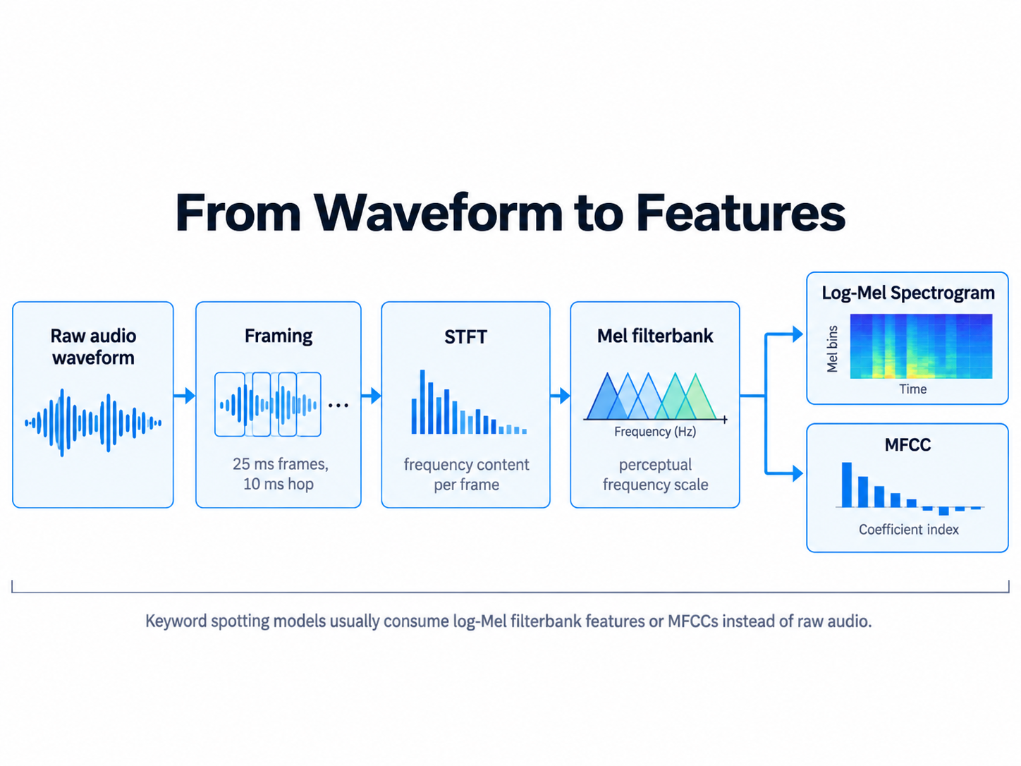
In the first step, the audio is divided into small overlapping frames, and in this, we have two things:
- frame size
- frame hop
Frame size is basically the number of samples in one single block, and frame hop is the number of samples that the window moves forward before taking the next frame, so it gives the flavor of an overlap.
For every frame, we compute its frequency content using the short-time Fourier transform. (read more - Short-Time Fourier Transform Explained Easily)
After this, we get to know how strongly different frequency components are present in each frame, but we, as humans, don't perceive frequency linearly. The difference between 200 Hz and 400 Hz is much more significant than the difference between 7,000 Hz and 7,200 Hz. This is why speech systems map the frequency onto a scale called the mel scale.
where f is the frequency in Hz and m is the frequency on the Mel scale.
Then we apply a series of triangular filters, which we call a Mel filter bank.
The way we apply these filters is we take a dot product of this with the power spectrum of the audio frame and each of the triangular filters.
Now our perspective of loudness is logarithmic. That's why we will now take a log, and we get something called the log mel spectrogram matrix.
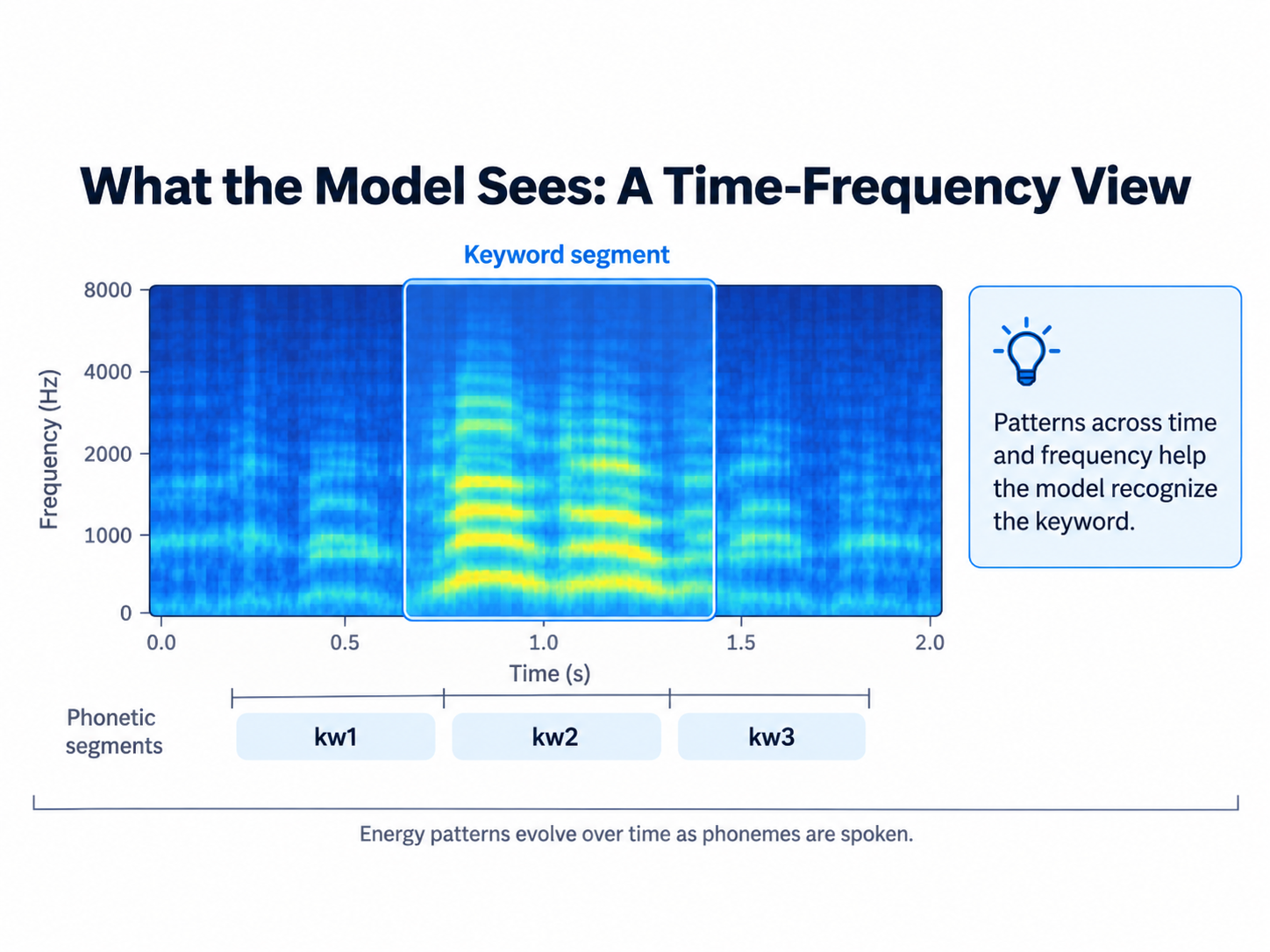
A spectrogram can be interpreted almost like an image. The horizontal direction is time, while the vertical direction is frequency. The intensity at each point is the amount of energy present in that frequency and time. Now, different phenomena will create different spectral patterns, and a keyword corresponds to a particular sequence of those patterns.
MFCC features
Another way to commonly represent, instead of the log mel spectrogram, is called mel frequency cepstral coefficients, or MFCC. MFCC compresses the mel spectrum into a smaller set of coefficients. Nowadays, people usually use the log mel filter bank because it gives richer time-frequency information, but in earlier cases, MFCCs were used.
The Neural Network
Once the features have been extracted, they are sent into a neural network. Suppose the target keyword is "hey device." The network is not programmed explicitly with the rules describing what individual phenoms will look like, so it learns from the examples.
"Hey Device" → keyword
"Hello Device" → not keyword
"Turn on the light" → not keyword
background noise → not keyword
music → not keyword
silence → not keyword
During training, the neural network tries to learn the acoustic patterns which are strongly associated with the target phrase. The output looks something like \(P(\text{keyword}\mid X)=0.97\).
To detect, we put a threshold. We try to detect if \(P(\text{keyword}) > Threshold\)
Models used in KWS
Many different methods can be used. We will discuss some of them.
Fully Connected
Early neural KWS systems often used dense neural networks. These networks were computationally cheap, but they did not explicitly exploit the local structure that is present in the time-frequency features.
Convolutional Neural Networks
The CNNs became very popular for keyword spotting. The spectrogram usually has the form \(X \in \mathbb{R}^{T \times F}\), Which can easily be processed to an image, so the convolution filters learn small local patterns across time and frequency.
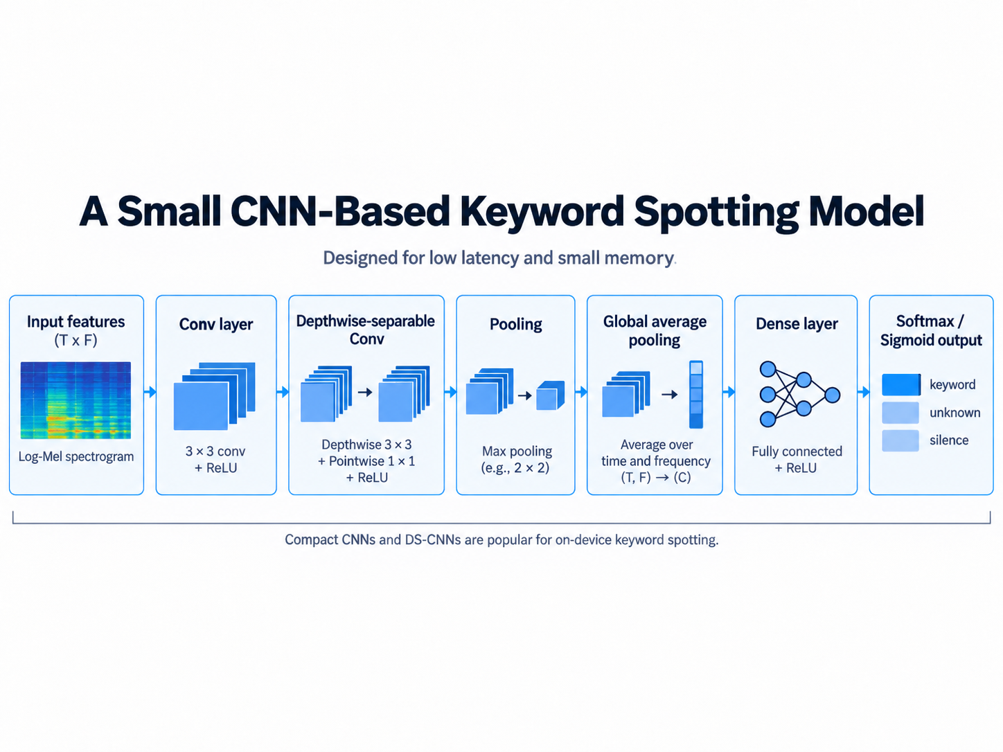
Convolution operation is roughly —
The filters learn usual local structures inside the spectrogram. In the case of speech, these structures might be frequency transitions, local phoneme patterns, or formant structures. This is the main reason that CNNs work particularly very well for keyword spotting.
Depth Separable Convolutional Neural Networks
For very small edge devices, standard convolutions are still very, very expensive. One popular alternative is the depthwise separable convolution. (read more - Xception: Deep Learning with Depthwise Separable Convolutions) Instead of performing one large convolution operation, the operation is separated into two parts:
- Depthwise convolution
- Pointwise 1x1 convolution
A normal convolution requires \(HWC_{in}C_{out}K^2\) total operations.
But a depth-wise separable convolution roughly requires $`HWC_{in}K^2
HWC_{in}C_{out}`$ operations, Only in the case where c_out and k are sufficiently large does it become comparable. That's why DSCNN architectures are commonly used for tiny word spotting systems.
RNNs, LSTMs and GRUs
Speech has a beautiful property that it is inherently sequential. RNNs process audio over time while maintaining one small internal hidden state. The equation of it comes out to be
The hidden state allows information from earlier frames that can influence later frames. LSTM/GRUs is an advanced form of RNNs only. (read more - RNNs [Week 4] - neuralnets)
CRNNs
Convolutional recurrent neural networks are the combination of the ideas of CNNs and RNNs. The CNN will extract the local acoustic patterns, and the recurrent layers then model how those patterns evolve over time. It's kind of like a CNN followed by an RNN.
Training a Keyword Spotting Model
A KWS training set usually contains several categories of audios. The main categories are —
Positive examples
Target keyword

Negative examples
Other speech

Background examples
Noise / silence / music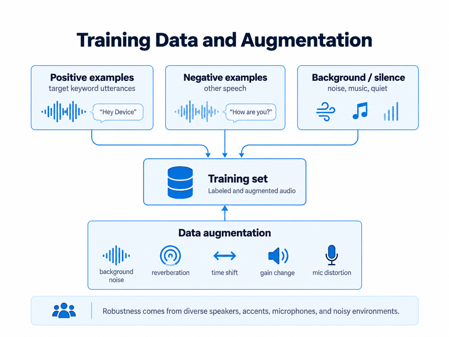
A binary system could use 1 whenever there is a keyword and 0 whenever there is not a keyword. You can also train it using binary cross-entropy, but many KWS systems use multiple classes, such as unknown, keyword, and silence. This unknown category is the most important thing. Without it, the model may be good at separating the keyword from silence but accidentally activate on very similar phonetic words.
Data Augmentation Is Extremely Important
The real-world data is a very messy thing to get into. We cannot assume that the user will speak directly into a very fancy $200 studio microphone, so the keyword may be spoken quietly, loudly, in a very noisy room, or in various kinds of scenarios. Hence, the training data will need a lot of augmentation to go with it. One simple augmentation technique can be mixing noise.
There are many ways to do it. You could add random gain. You could do pitch variation, and there are many ways to do data augmentation in this case.
Continuous Detection
Training a classifier is only one small part of the problem. When you deploy this model, the model runs repeatedly on overlapping windows. Suppose the system produces —
| Time | P(keyword) |
|---|---|
| 0.0 s | 0.04 |
| 0.1 s | 0.08 |
| 0.2 s | 0.12 |
| 0.3 s | 0.31 |
| 0.4 s | 0.67 |
| 0.5 s | 0.91 |
| 0.6 s | 0.96 |
| 0.7 s | 0.94 |
| 0.8 s | 0.71 |
| 0.9 s | 0.28 |
A naive detector will just simply trigger whenever it crosses the threshold values, but it will now create false activation because one noisy window could give a very high prediction value. Hence, we need smoother predictions. One simple experimental smoothing rule is
where:
- \(p_t\) is the current prediction
- \(s_t\) is the smoothed prediction
- \(\alpha\) controls how quickly the score changes
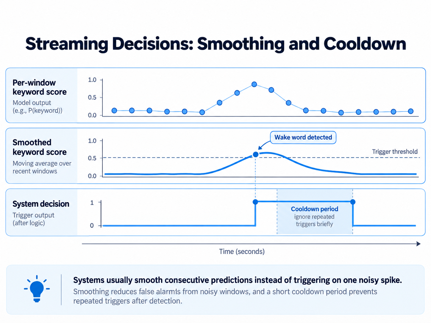
So instead of reacting to one isolated spike, the system will now require the confidence to remain high across many consecutive windows. If there is smoothing, we can now actually eliminate a lot of false positives.
Cooldown and Debouncing
Suppose the model detects a device. Because the sliding window overlaps, many consecutive windows may contain nearly the same word, so without additional logic, the system will not trigger multiple times.
Window 101 → trigger
Window 102 → trigger
Window 103 → trigger
Window 104 → trigger
So, to prevent this, the system enters a small cooldown period after it detects, like 1 second or something. This mechanism is very similar to the concept of debouncing in real-time systems.
False Accepts vs False Rejects
One of the most important problems here is selecting the detection threshold. There are these two main failure modes.
False Accept
The system will activate even though the keyword was never spoken. The user might say, "I really like that device," and the system activates accidentally, even though the word "hey device" was never spoken.
False Reject
When this is exactly the opposite case where the user actually says "hey device," but the system will not activate
Now you would notice that there is a trade-off between these two errors.
A low threshold will mean:
- Higher sensitivity
- Fewer missed keywords
- More accidental activations
A high threshold will mean:
- Lower sensitivity
- Fewer accidental activations
- More missed keywords
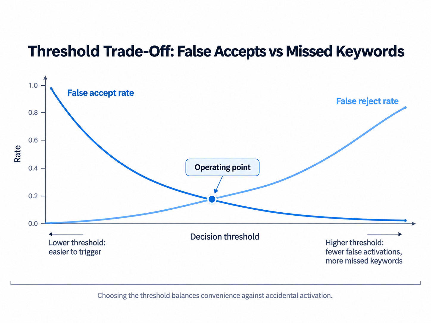
So here, we have to do this: there is a metric called false activations or false rejects per hour. We monitor that to actually find the threshold. This will matter because of the time concept. These models will operate continuously, so even if the false positive rate looks extremely small per prediction, it can become very significant when the model is performing millions of predictions over the hour.
Why are these models tiny?
Wake word detection is an always-on workload problem. The model has to run 24 hours a day, 7 days a week, so this changes the optimization problem in a different kind of way. A large ASR model can consume a substantial amount of compute when the user explicitly activates it.
But this detector cannot. It must continuously monitor audio while consuming very little energy, so we must focus on:
- Low latency
- Low power
- Small memory
- Small model size
- Real-time inference
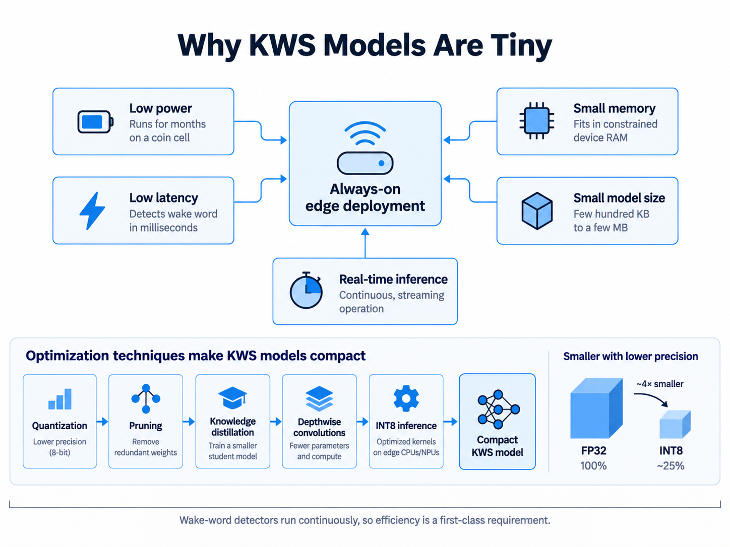
You can also make the model smaller by methods like quantization, pruning, distillation, and so on.
Why Keyword Spotting Is More Difficult Than It Looks
At first glance, this problem appears to be a simple classification problem. You get the audio, and you just judge: is it a keyword or not a keyword? But a real-time system has to solve a much harder problem in depth.
It has to have a low false activation rate, low latency, low memory, and low power consumption while being robust to music, traffic, background conversations, and all kinds of different noise.
The model can even work on the developer's device and achieve excellent test set accuracy, but still be completely usable on the user's device. That's why production-level keyword spotting models are less about maximizing ordinary classification accuracy, and it's more about designing this end-to-end system to work perfectly.
Finally
What makes keyword spotting interesting is not the optimization part of it. It's quite the opposite, I feel. The challenge is building the model that will contain only a few hundred thousand parameters, run continuously on extremely constrained hardware, respond almost instantly, and can listen for months and years without constantly activating by mistake.
This weird concoction of signal processing, neural networks, streaming systems, hardware constraints, and statistical decision-making is what makes this problem one of the most interesting practical problems in edge machine learning.