Basics of NLP - 2 [Week 6]
discussion into how pos tagging, ner, sentiment analysis, and n-gram models work
We have covered some of the basics in part 1 of this series
Check that out : Basics of NLP - 1 [Week 5]
Let’s continue from where we left off.
This blog is broken into 4 pieces
- Part-of-Speech Tagging
- Named Entity Recognition (NER)
- Sentiment Analysis
- N-grams
Part of Speech Tagging
The basic understanding is that we label each word in the sentence with its corresponding parts of speech. A part of Speech is a category of the word we assign to a type of word in a sentence, for example, cat is a noun, or go is a verb.
It is mainly a preprocessing step before applying earlier techniques.
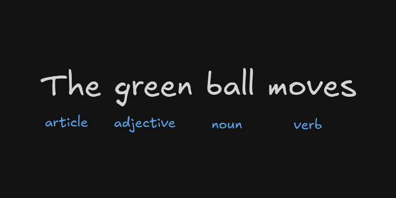
How does it work?
We will find out the POS tagging for the sentence Will will eat apple
For that, we need first to take some sample sentences and do POS tagging on them.
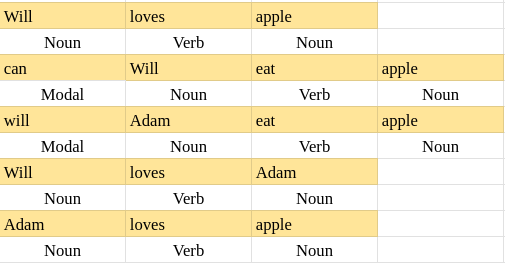
Now we need to make an emission probability table first, let’s learn while building it.
| Unique Words | Noun | Verb | Modal |
|---|---|---|---|
| Adam | 2/8 | 0 | 0 |
| will | 3/8 | 0 | 1/2 |
| apple | 3/8 | 0 | 0 |
| eat | 0 | 2/4 | 0 |
| can | 0 | 0 | 1/2 |
| loves | 0 | 2/4 | 0 |
We just count the frequencies of in what context they have been used in the sentences and find their probabilities concerning the part of speech (column-wise).
Now we build a transition probability table. For this, we add a start and end tag before the sentences.
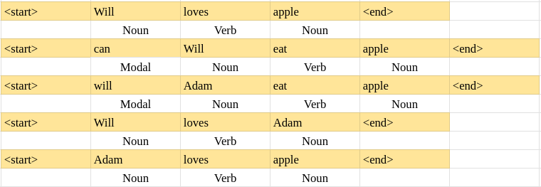
| Noun | Modal | Verb | End | |
| Start | 3/5 | 2/5 | 0 | 0 |
| Noun | 0 | 0 | 5/10 | 5/10 |
| Modal | 2/2 | 0 | 0 | 0 |
| Verb | 5/5 | 0 | 0 | 0 |
Now we make something called a Hidden Markov Model.
More about Hidden Markov Models
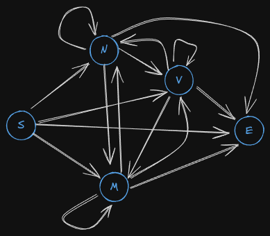
Now let’s revisit our first statement, Will will eat apple
Let us consider all of them nouns and fill in the emission and transition probabilities.
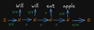
The total probabilities come out to be 0. Hence such a part of speech tagging is completely impossible.
Now we change the parts of speech and find probabilities in all the cases. In this case, there will be \(3^4 = 81\) cases in total. There will be more, so how can we optimize this process?
Viterbi Algorithm
This is the algorithm that will let us know the correct part of speech. Let us first consider all the probabilities and then see the first pass ( Start → Noun/Verb/Modal)
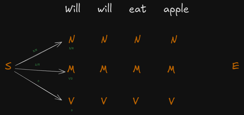
From this we know Verb after Start is impossible, so we don’t consider it at all. Will can be either Modal or Noun, let’s see the next pass.
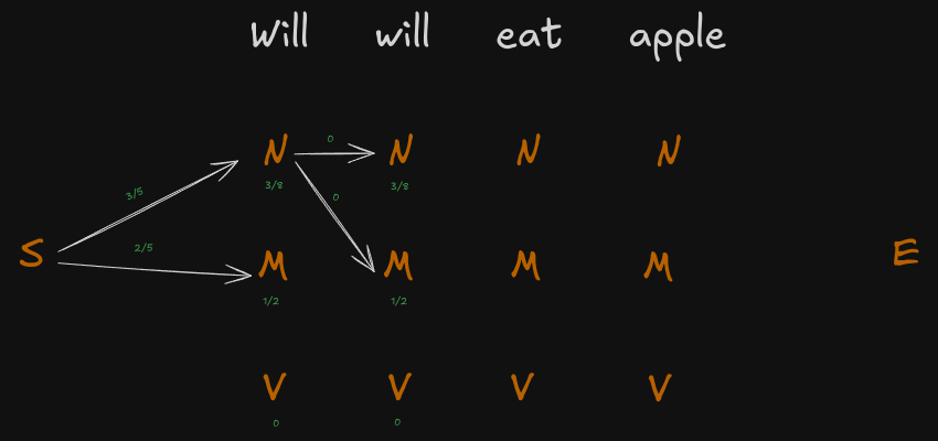
Hence, Will can’t be a noun in the first case at all. Let’s see its pass for Modal now.
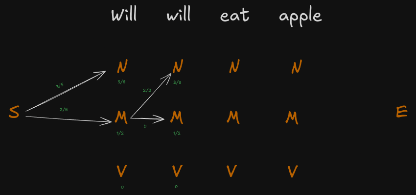
Hence clearly from this, we get to know that Will will be a modal followed by will being a noun.
We carry on doing this till we reach the end. Finally the diagram will look something like this.
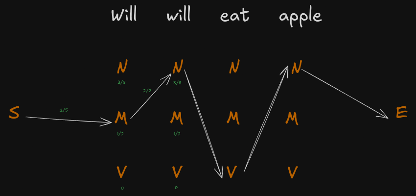
Hence the part of speech tagging is done as follows :
| Will | will | eat | apple |
| Modal | Noun | Verb | Noun |
Why do this?
- This forms the basis of named entity recognition(NER), which we will look into in the next part.
- It is used in a lot of chatbots.
- It can help to differentiate between the meaning/context of words, like
go left- left is a noun here, meaning directionsI left- left is a verb here, meaning exiting
Named Entity Recognition(NER)
In this, we first need to define an entity. Entity here is nothing but a simple class/type of any object. For example, a Company is an entity and it will have objects like Google, Apple, etc. under it.
How does it work?
Let us try to understand how this works. Let’s take a sentence and a few entities.
Sentence - neuralnets went to buy Boat earphones from Sarojini Market on 6th December
Entities - Name, Location, Company, Date
Preprocessing and Entity Identification
First, we will do text preprocessing, as we have discussed earlier (mostly tokenization is used).
After that, we try to identify which of the words are an entity and which aren’t.
For example, we can notice that went will not be an entity, while my name neuralnets will be an entity. How do we do this?
As you saw we had first done tokenization, then we did feature extraction on it to understand the significance of each token. We check its morphological features, like root forms, then check it’s semantic features that capture the meaning of words, and many more to find out how much a token is significant in that context.
Entity Classification
There are several ways to do this, let’s discuss a few of them:
- Lookup of Data
In this, we just look up the data in already available databases. To label Boat as a company, I will have to search all the databases of
Name, Location, Company, and DateforBoatand then label it as aCompany.
This is very time and resource-hungry, hence we don’t do this in real life. - Rule Based Approach
We define some rules for the computer to label something as an entity. For example, let’s make a rule that any word after
onis a Date, hence6th Decemberwill be labeled as aDate. This also is not that practical, hence we don’t use this much. - Statistical Approach
We can also employ statistical models such as the Hidden Markov Models taught earlier to find out the correct entities.
- Machine Learning Approach
You can use SVMs and Decision Trees to label data to their named entities. These stuff need a lot of labeled data themselves to train hence we now use other methods to substitute them. Recurrent Neural Networks and Transformers have become the household name for NER recognition now due to their ability to do large-scale tasks with abundant training data.
Why do this?
- Resolves ambiguity in words, like the word
Appleis both a company and a fruit. Thus labelling it removes all the confusion - Provides the necessary context in which it is used,
I went to the Amazonrefers to the jungle whileI work at Amazonrefers to the company. Context gets resolved due to NER
Exercise - Create a fun resume analysis tool that will automatically shortlist candidates based on some predetermined skills. Use NER to do it.
Sentiment Analysis
In this kind of analysis, we try to find out what the sentence is feeling overall. For example,
I am feeling great is a positive sentiment, while I am dying is a negative one.
How does it work?
Let us try to find out the sentiment of the sentence predictable with no fun
First, we need some training samples, with their sentiments
| Sentiment | Sentence |
|---|---|
| Positive | the most fun film of the summer |
| Positive | very powerful |
| Negative | no surprises and very few laughs |
| Negative | entirely predicatable |
| Negative | just plain boring |
First, we do text preprocessing and remove the non-important words from our target, which then becomes predictable no fun
A simple way of doing sentiment analysis is trying to just see the probability of a sentence being negative or positive
So we use the method of Naive Bayes to solve this sentiment analysis issue, we first calculate the probability likelihood of each case, using this formula.
How did we get this?
Now we find all the probabilities of predictable no fun with respect to all sentiments.
Now we see the total probability of the sentence S = predictable no fun.
Now we find out the scores of the sentence S now
We see that S being a negative sentiment has a higher probability, hence S must be a negative sentiment.
We can do this for more sentiments too, I took a smaller example for an easier example.
Optimizations
We can notice that the occurrence of the word great tells us it is a positive sentence, but its appearance 6 times doesn’t contribute too much. Hence we can do something like this. So we clip out word counts at 1, if like a word occurs 5 times, we pretend it appeared once, and perform Naive Bayes as above.
This kind of optimization is called Binary Multinomial Naive Bayes.
Exercise - Create a sentiment analysis tool that divides sentences into sentiments of happy, sad, angry, and no emotion.
N-Gram Models
Let’s say we have a part of a sentence - This is a ___
What will be the next word here?
This is what n-gram models help us to find.
n-grams are sequences of n-words together with each other. Let’s take an example of a 4-gram.
We need to first have a corpus of text
Corpus
This is the house that Jack built.
This is the malt
That lay in the house that Jack built.
This is the rat,
That ate the malt
That lay in the house that Jack built.
This is the cat,
That killed the rat,
That ate the malt
That lay in the house that Jack built.
What is the \(P(house | This \space is \space the )\)?
This is the will be in Sentence 1,2,4,7, and This is the house is in Sentence 1, thus making the probability to be \(\frac{1}{4}\).
We can also test for a bi-gram from this. Let’s try to find out \(P(that Jack|that)\)
We can easily see the answer to be \(4/10\)
How does it work?
Let’s predict the probability of a sequence of words.
We will apply the chain rule to this :
To compute the larger terms at the end like \( p(w_k|w_1 \dots w_{k-1})\), it is very complicated as you have to recompute the probabilities of each word every time. Hence we use the Markov Assumption. It tells us we don’t need to calculate from \(w_1 \) to \(w_{k-1}\) as it is very unlikely that all of the text is connected to itself.
Bigram Language Model
The equation becomes this in the case of bigram model(n=2).
Let’s take an example, let’s take a corpus
This is the malt
That lay in the house that Jack built
Now let’s find out \(P(this\space is \space the \space house)\)
There are two problems,
- We should not use the probability of \(w_1\) distributed throughout the corpus, but instead only use the start words.\[p(w) = p(w_1|start)p(w_2|w_1) \dots p(w_k|w_{k-1})\]
- The same needs to be done at the end too.\[p(w) = p(w_1|start)p(w_2|w_1) \dots p(w_k|w_{k-1})p(end|w_k)\]
In short, we can conclude bi-gram models to be :
Why do this?
- Used in Autocorrect
- Used in Machine Translation
- Used in Speech/Handwriting Recognition